A Finite Element Method
Based
CFD Program
Contact: cfd-rocket@gmail.com
Chapter 1. Introduction
The FluSol is a general purpose finite element method based, unstructured grid compressible flow computer program. It uses the two-step Taylor Galerkin finite element method to solve the inviscid and the viscous flow equations with or without chemical reactions. In additional to solve the above Euler and Navier Stokes equations, the same finite element method was successfully applied to solve the inviscid/viscous conical flow equations. The program can also solve the two phase flow problems of air and small solid particles mixture, both the Eulerian-Eulerian or the Lagrangian-Eulerian approaches are available.
For mesh generation, FluSol uses text based scipts (.msh file) to generate hybrid triangle and quadrilateral elements for 2D computational domain and hybrid elements of hexahedrons, prisms, pyramids, tetrahedrons for 3D computational domain. It can also convert any 2D mesh built by all quadrilateral elements into all triangle elements and any 3D model built by all hexahedral elements into all prisms or pyramids or tetrahedrons. By sweeping the 2D mesh around the axisymmetric line plus pre-specified number of wings and wing cross-section shape, a 3D mesh for wings and body combinations can be easily generated within seconds. The generated 3D meshes will consist of the hexahedral, prisms, pyramids and the tetrahedral. All necessary information, such as boundary conditions, initial conditions, solid wall and farfield conditions will also be written into this generated 3D mesh file. Users can run the solver immediately after the mesh file was generated.
1.1
Capabilities
Table 1.1 shows the program’s current capabilities.
|
|
Structured or Unstructured |
Hybrid Grids |
Unsteady State Solution |
Steady State Solution |
Viscous Flow |
Inviscid Flow |
Chemical Reaction |
|
1D Plannar
Flow |
Yes |
No |
Yes |
Yes |
Yes |
Yes |
Yes |
|
1D Cylindrical Flow |
Yes |
No |
Yes |
Yes |
Yes |
Yes |
Yes |
|
1D Spherical Flow |
Yes |
No |
Yes |
Yes |
Yes |
Yes |
Yes |
|
2D Plannar
Flow |
Yes |
Yes |
Yes |
Yes |
Yes |
Yes |
Yes |
|
2D Axisymmetric Flow |
Yes |
Yes |
Yes |
Yes |
Yes |
Yes |
Yes |
|
3D Flow |
Yes |
Yes |
Yes |
Yes |
Yes |
Yes |
Yes |
|
3D Conical Flow |
Yes |
Yes |
No |
Yes |
Yes |
Yes |
No |
|
Two Phase Flow |
Yes |
Yes |
Yes |
Yes |
Yes |
Yes |
No |
Table 1.1 Capability Table For Compressible Flow
Chapter 2
Governing Equations and Finite Element Formulation
2.1 Governing Equations
The three dimensional Navier-Stokes and species transport equations for a chemically reacting gas of N species are given by
 (2.1.1)
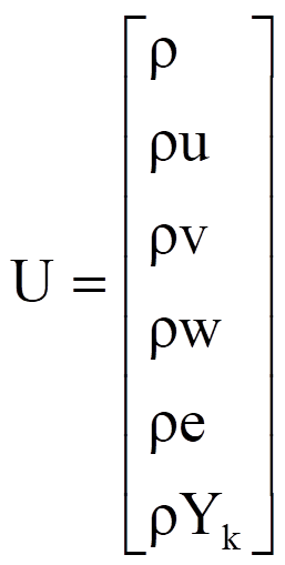
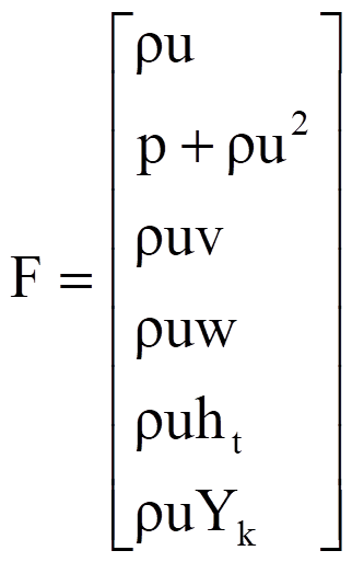
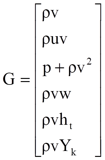
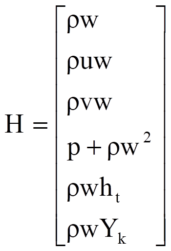
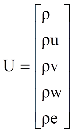
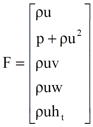
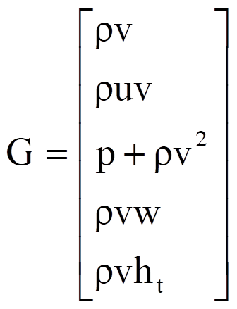
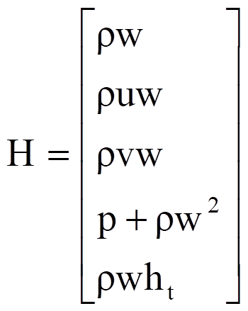
Where U is the conservative vector, F ,G, and H are inviscid flux vector and Fv, Gv, and Hv are the viscous flux vector. S is the source term vector. U, F, G, H, and S are defined as follow :
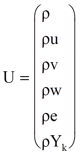
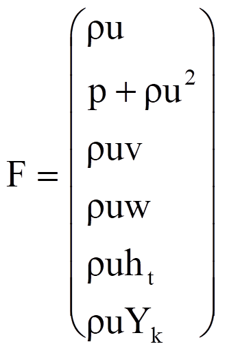
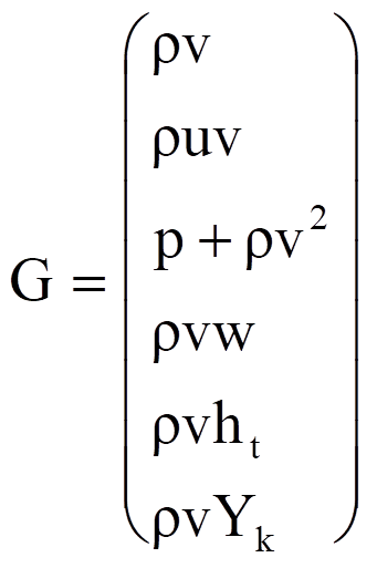
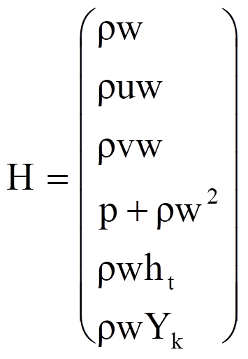
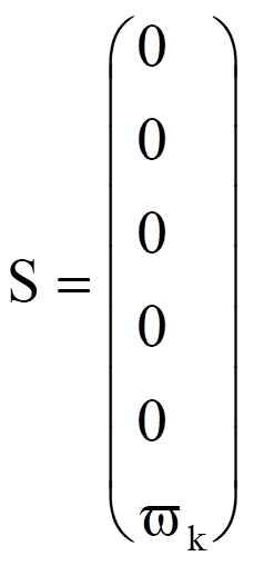 (2.1.2)
Here u, v and w are velocities. r and p are the density and pressure of gas. Yk is the mass fraction of k species. ht is the total enthalpy consists of gases thermal and chemical energy plus kinetic energy.
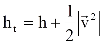 (2.1.3)
et is the specific total internal energy.
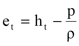 (2.1.4)
The viscous flux Fv, Gv, and Hv are defined as:
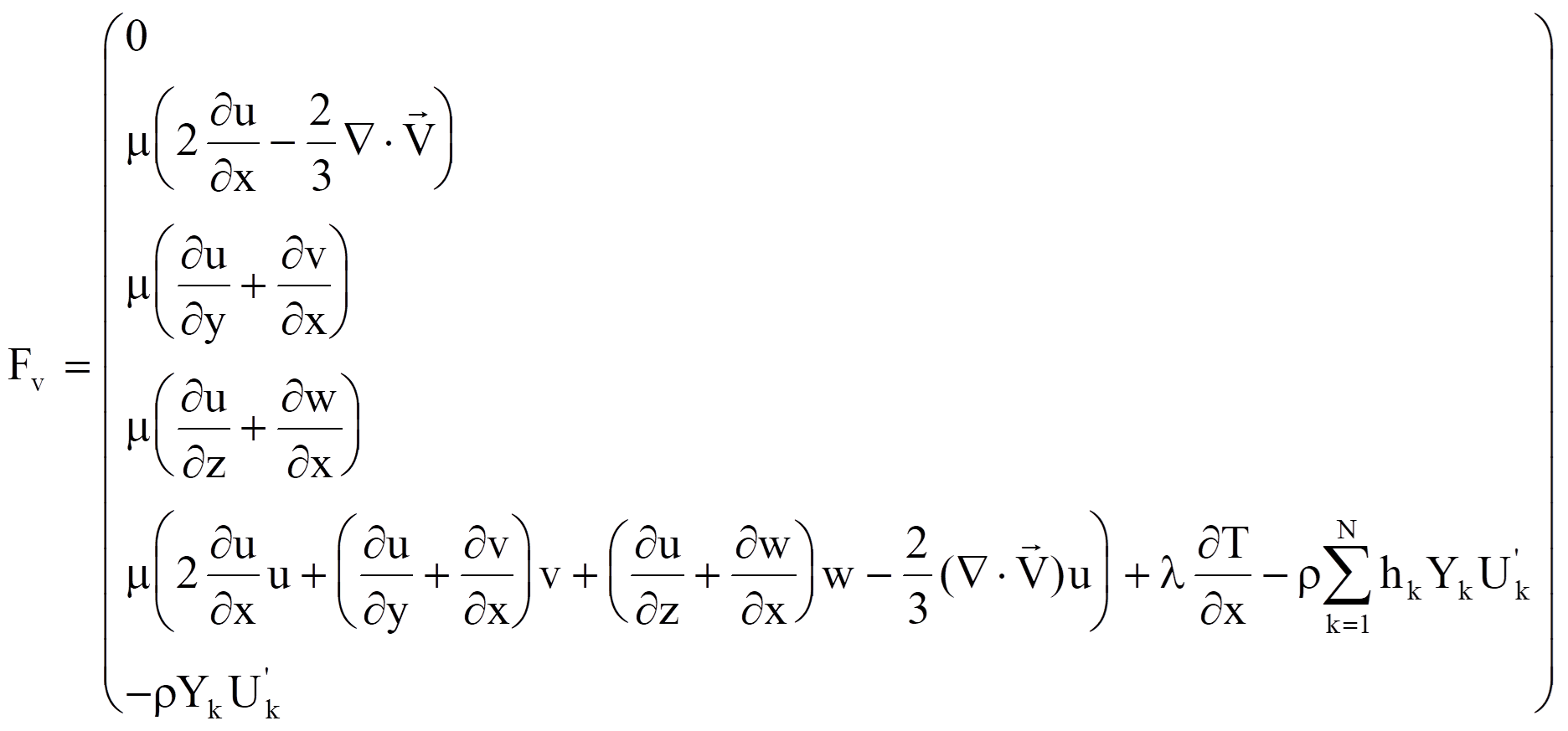
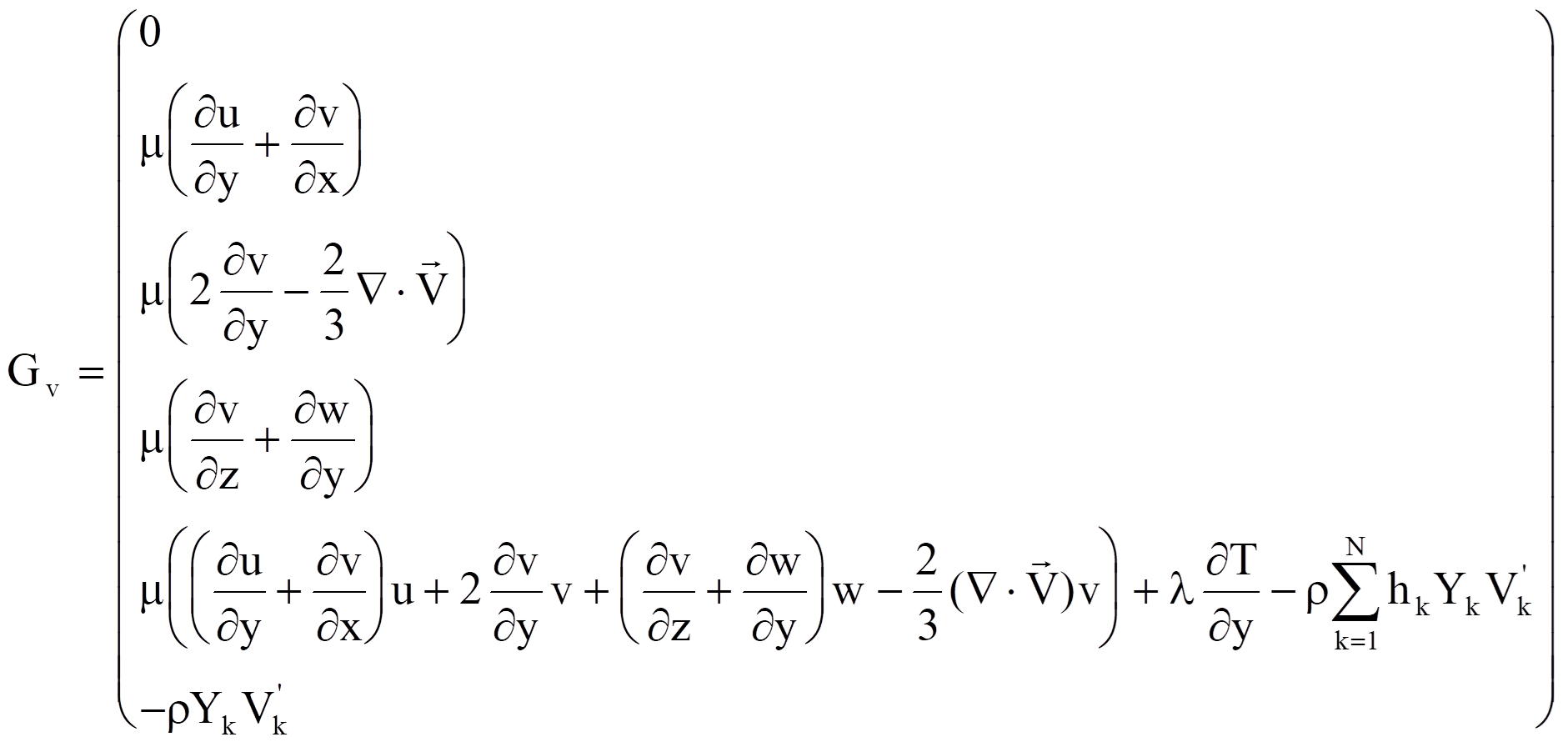
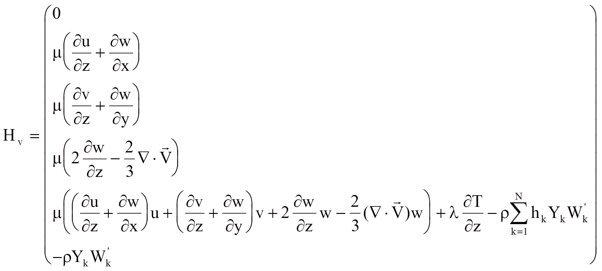

For multiple components chemically reacting flow, the FluSol program incorporates a chemical kinetics package Chemkin [Kee 1991] and a transport property package Transport [Kee 1986]. These two packages perform all chemical reactions and calculate all species and mixture thermodynamic and transport properties such as specific heat, internal energy, thermal conductivity, viscosity, mass diffusion coefficients .... etc. The theory and formulations used in these packages are briefly summarized as below. For detail information, users are suggested to read corresponding manuals. In the present application of above packages, the idea gas mixture equation of state is assumed and defined as :
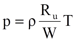 (2.1.5)
Where Ru is the gas universal constant and W is the mean molecular weight that is related as to the individual molecular weight Wk of species k by :
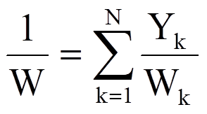 (2.1.6)
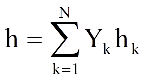
The specific mixture enthalpy h is defined as :
 (2.1.7)
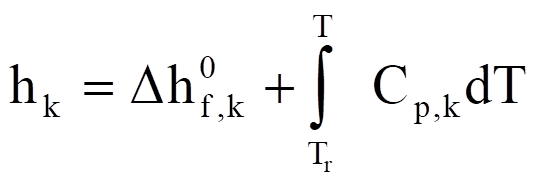
with the specific enthalpy of species k given by
 (2.1.8)
Where 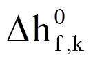 is the standard
enthalpy of formation at reference temperature Tr.
The constant-pressure specific heat for each species is calculated according to
a fourth order polynomial of temperature :
 (2.1.9)
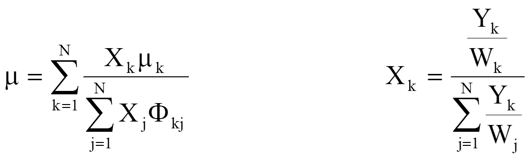
Where Rk is the gas constant of species k and a1k,...,a1k are constant coefficients. The viscosity and thermal conductivity of the individual species are estimated by standard kinetic theory [Hirschfelder et al. 1954; Warnatz 1982]. The mixture viscosity is then determined by the semi-empirical Wilke [1950] formula modified by Bird et al. [1960]
 (2.1.10)
Where Xk is the mass molar fraction of species k and Fkj is defined below :
 (2.1.11)
The mixture thermal conductivity is evaluated by an averaging formula [Mathur et al. 1967]
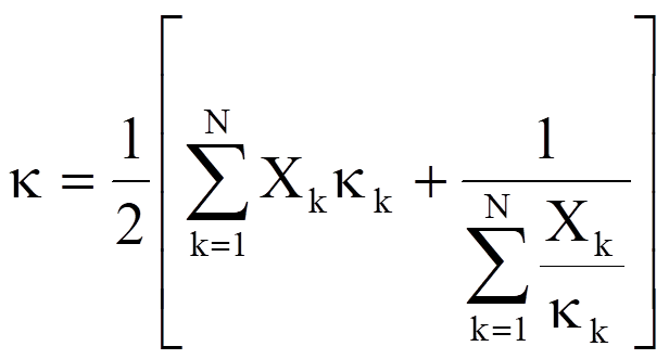 (2.1.12)
In the above expression Xk is the mole fraction of species k in the gas mixture. The molecular binary mass diffusion coefficient Dij between species i and j is obtained by using the Curtiss-Hirschfelder approximation [Hirschfelder et al. 1954]. For simplicity, the species mass diffusion in the gas mixture is approximated by Fick's law and the diffusion velocity is calculated by
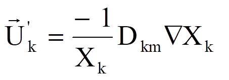 (2.1.13)
Where Dkm is the effective binary diffusion coefficient of species k in the gas mixture. Dkm is obtained by treating the species k and the surrounding gas as a binary system. Dkm is given by Bird et al. [1960],
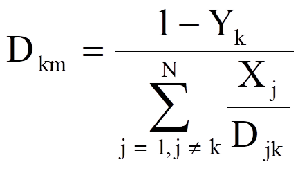 (2.1.14)
It should be pointed out that the Fick's law is just a convenient approximation to the exact multicomponent diffusion equations derived from molecular kinetic theory. If an accurate diffusion velocity is desired, the multicomponent diffusion equations should be used. In additional to above transport properties, the mass production rate expressions for the chemically reacting flow still needed to be defined. For L elementary reversible or irreversible reactions involving N chemical species, the chemical equations can be expressed by :
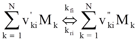 i =1,2,...,L (2.1.15)
where vki is the stoichiometric coefficient of the k-th species in the i-th reaction, mk is the chemical symbol for the k-th species, and L is the total number of reactions. The prime and double prime denote the reactants and products, respectively. The net mass production rate wk of the k-th species can be written as a summation of k-th species production rates for all reactions involving the k-th species :
 (2.1.16)
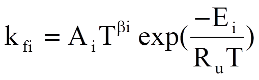
Where Cj is the molar concentration of the j-th species and kfi and kri are the forward and the reverse rate constants of the i-th reaction. The forward rate constants for the L reactions are generally assumed to have the following Arrhenius form :
 (2.1.17)
where the pre-exponential factor Ai, the temperature exponent bi, and the activation energy Ei should be specified by the user. The reverse rate constants kri are related to kfi through the equilibrium constants Kci as :
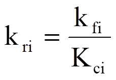 (2.1.18)
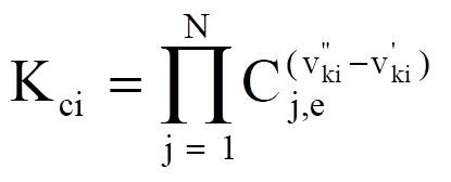
with
 (2.1.19)
Where Cj,e denotes the equilibrium molar concentration of species j. In additional to the standard Arrhenius form for reaction rate constants, Chemkin package can handle some special rate expressions. Those expressions are the third body reaction, the pressure dependent fall of reaction [Lindemann form, Toe form and SRI International form], and the Landan-Teller reaction [Kee et al. 1991].
2.2 Non-dimensional form
The governing equations are often put into non-dimensional form. The advantage of non-dimensional form is the characteristic parameters, such as Reynolds number, Prandtl number, etc., can be varied independently. Also, by non-dimensionalizing the governing equations, the flow variables are normalized so that their values fall between certain prescribed limits such as 0 and 1. Inside the program the non-dimensional form of equation (2.1.1) is used. The non-dimensional form of equation (2.1.1) is obtained by the following procedure :
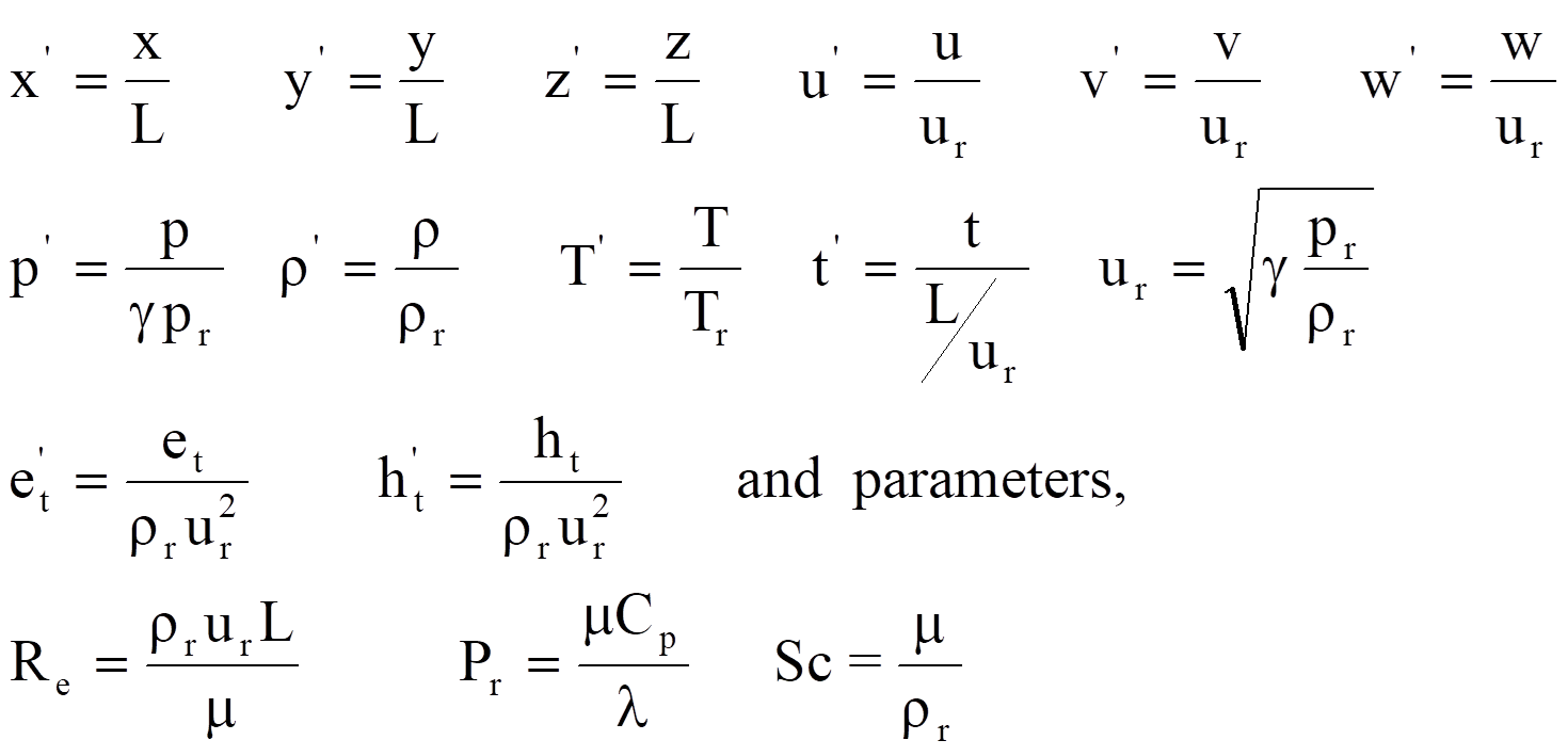 (2.2.1)
After substituting above non-dimensional variables into equation (2.1.1) and dropping superscripts " ' ", the non-dimensional form of equation (2.1.1) can be expressed as :
 (2.2.2)
Where Re is the Reynolds number, the non-dimensional flow variables and inviscid fluxes terms are defined as
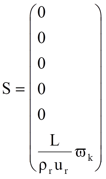
The viscous flux can be expressed as :
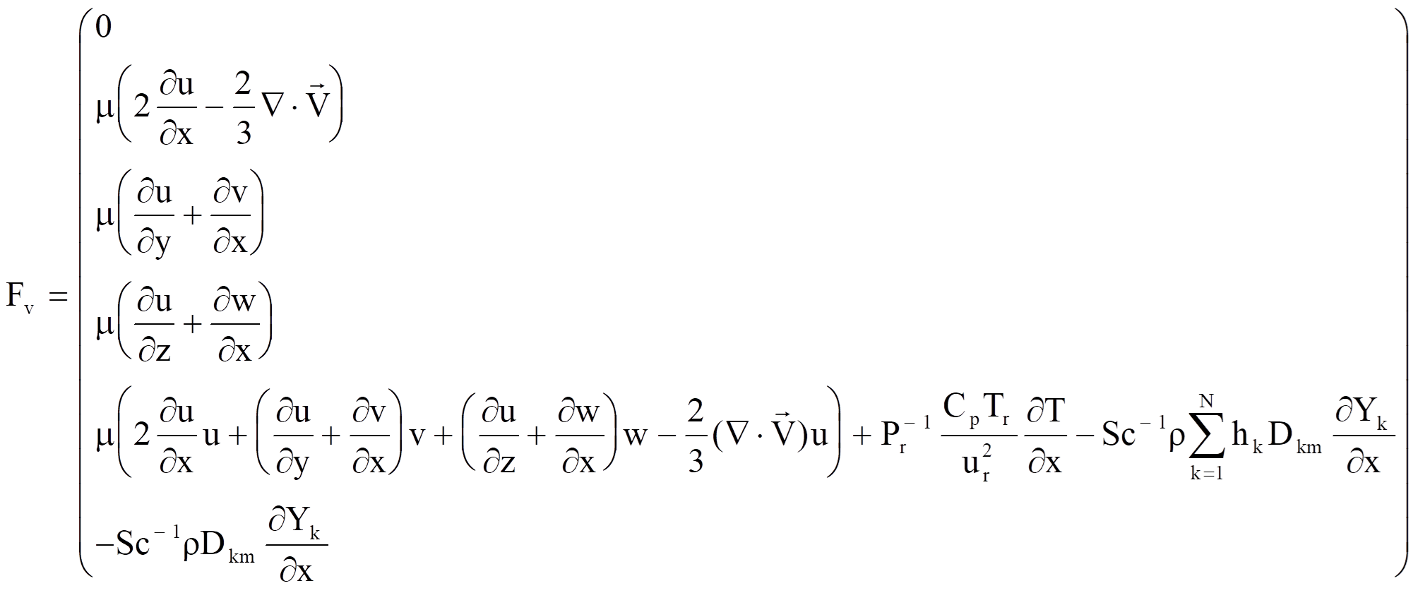
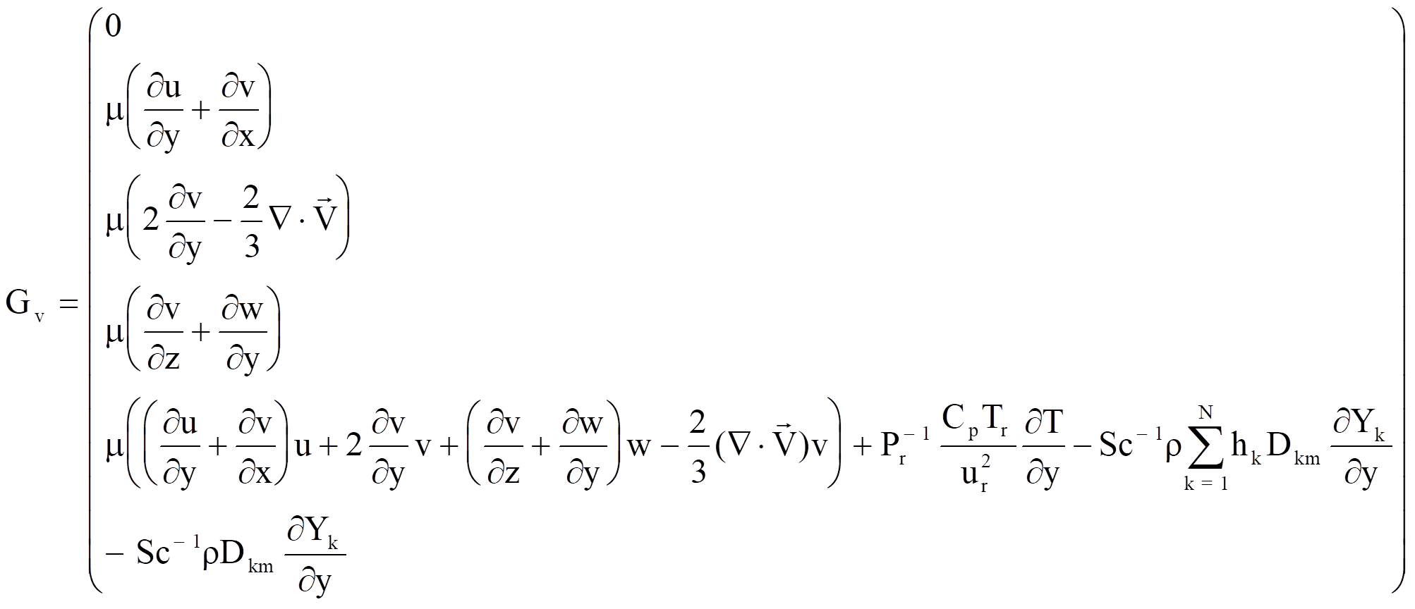
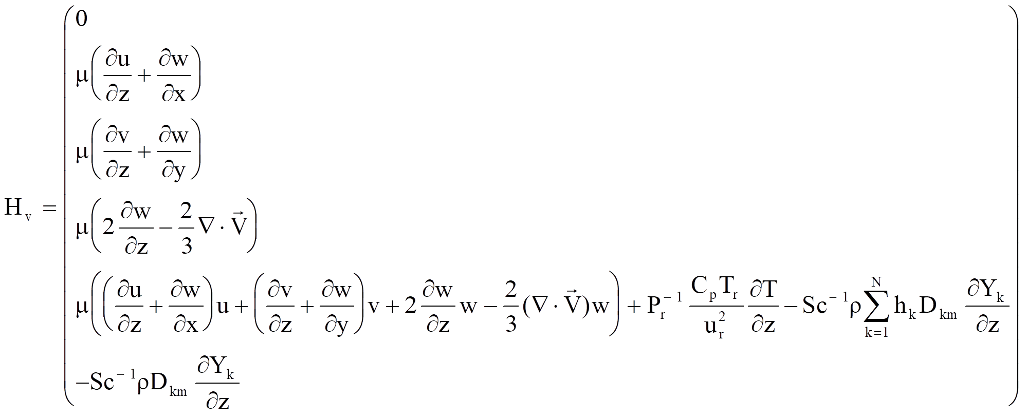
2.3 Compressible Navier Stokes equations
The above governing equations can be simplified into the pure gas Navier Stokes equations. If the flow is only single component without chemical reaction and no mass diffusion, then the species equations can be eliminated and the inter-diffusion energy flux terms in the energy equation can be dropped. Equation (2.2.2) will become :
 (2.3.1)
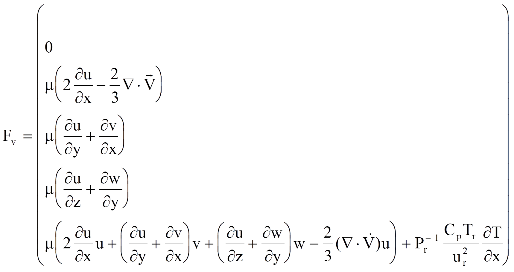
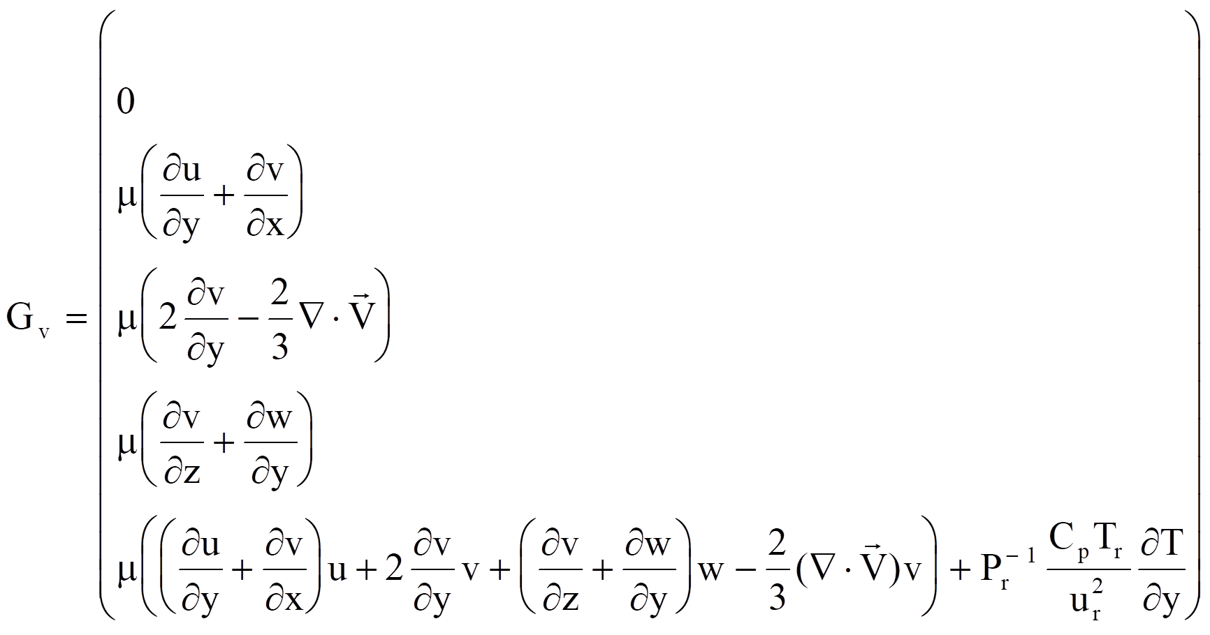
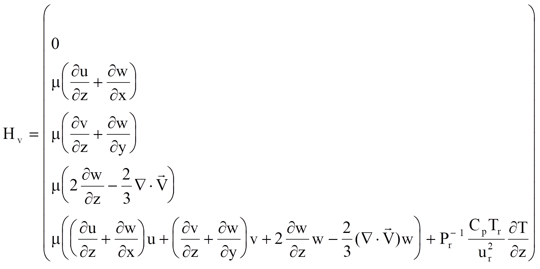
For non-reacting flow usually the specific heats Cv and Cp are constants, then the total energy et can be expressed as :
 (2.3.2)
The viscosity m can be evaluated by the Sutherland law.
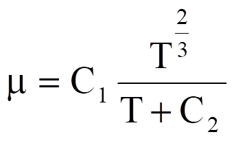 (2.3.4)
Where C1 and C2 are
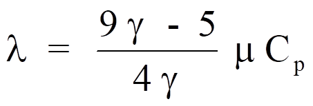
constants for a given gas. For air at moderate temperatures, C1 =1.458x10⁻⁶ kg/(ms oK1/2) and C2=110.4 oK. The thermal conductivity l is then evaluated by Euken
formula :
 (2.3.5)
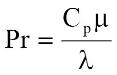
Following the above formula, the Prandtl number defined below :
 (2.3.6)
is Pr = 2/3 for monatomic gases ( g = 5/3) and Pr = 14/19 for diatomic gases. The latter value is a good estimate for air.
2.4 Euler Equations
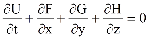
If all viscous and heat transfer terms in equation (2.3.1) are dropped, then the resulting equation is called the Euler equations. The Euler equations can be solved using much less computer time and memory than those required for solving the complete Navier Stokes equations.
 (2.4.1)
with
2.5 Initial and Boundary Conditions
For a problem to be well defined, proper initial and boundary conditions must be specified in additional to the governing equations. A user must provide initial values for all flow variables on the whole computational domain for his particular problem. Specifically the user needs to specify velocities, pressure, density, and species mass fractions; if it is a multiple component problem, on each node of the computational domain :
u,v,w,p,r,Y1,Y2,.....,YN
There are two types of boundary conditions for a typical compressible problem : farfield conditions and solid surface conditions. For farfield boundary conditions, there are four types of treatments :
1. At each farfield node a fiction element cell is created in the normal direction. The flow variables at this node are calculated by summation of all contributions from every element connected to this node.
2. Jamenson's approach [1986] of local one dimensional analysis of Riemann invariant normal to the outer boundary is used.
3. The same as method 2 but at subsonic exit locations free stream static pressure are kept constant.
4. The same as method 2 and 3 but at exit locations, zero gradients are applied.
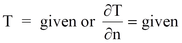
For viscous flow, the boundary conditions on the solid wall are the non-slip conditions. Also a first kind or second of temperature boundary condition is need to applied by the user. If it is a multicomponent flow, the wall is assumed to be non-catalytic. In this case the boundary conditions on solid wall can be expressed as
u = 0, v = 0, w = 0

2.6 Finite Element formulation
In the FluSol program, the two-steps explicit Taylor Galerkin finite element method is used to solve the above flow equations. A general Taylor series expansion of n+1 time step in terms of n time step can be expressed
 (2.6.1)
Where the superscript denotes the time level. This general form can also be achieved by a two-step scheme
 (2.6.2)
It can be seen from equations (2.6.1) and (2.6.2) that if Q1=1.0 then the final results for both equations are the same. The purpose of inserting the variable Q1 is that through the value of Q1 the order of time accuracy can be easily controlled by the user. The value of Q1=1.0 or Q1=0.0 determines the numerical scheme to be a second or first order time accuracy.
 (2.6.3)
When rewriting equation (2.2.2) at time level n and drops all viscous terms, equation (2.2.2) become
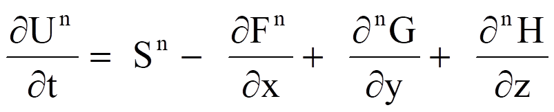 (2.6.4)
After substituting the time derivative term of equation (2.6.4) into equation (2.6.3), equation (2.6.3) becomes
 (2.6.5)
It should be noted that at the first time step viscous flux terms are not included. The reason is viscous flux terms are second order derivative terms in space. In the first time step, only element center values are calculated. Also in the present theory, only linear elements are considered. Therefore, the most order of accuracy in space can be achieved in the first time step is only the first order. To perform the finite element evaluation of the above equation, the following approximation are used
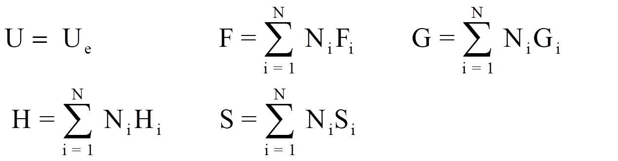 (2.6.6)
Where Ni is the linear shape function for the node j. After substituting (2.6.6) into equation (2.6.5) and integrate over each element volume. Equation (2.6.5) becomes
 (2.6.7)
It should be noted that Ue represents the flow variables at the element center. After finding Ue, then the value of Fe, Ge, and He can be found. For the second step, equation (2.2.2) can be rewritten as
 (2.6.8)
Second step :
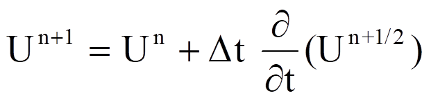 (2.6.9)
substitute equation (2.6.8) to equation (2.6.9), equation (2.6.9) becomes

(2.6.10)
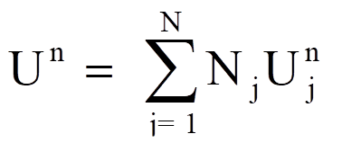
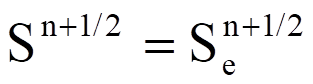
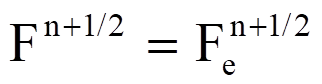
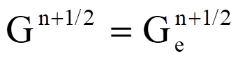
Un+1, Un, Fn+1/2, Gn+1/2, and Gn+1/2 are defined as :
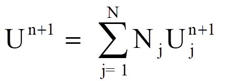
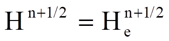 (2.6.11)
Multiply the weighting function Nk and substitute Un+1,Un, Fn+1/2, Gn+1/2, Hn+1/2, and Sn+1/2 of equation (2.6.11) into equation (2.6.10) and take integration over the all computational domain
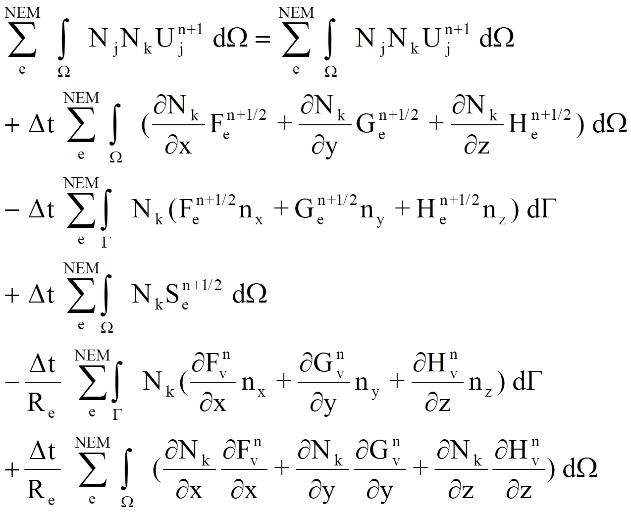 (2.6.12)
Where G is the boundary of the domain W. nx, ny, and nz are the direction consine of the outward normal to G. Equation (2.6.12) is a set of implicit linear algeraic equations. Since the left hand side matrix called consistent mass matrix is not a diagonal matrix. To solve equation (2.6.12), one must resort to the iterative method which is time consuming and demanding large computer memory. On the other hand, in many applications, the consistent mass matrix had been simplified by replacing it with a lumped, diagonal mass matrix Md whose diagonal entries are defined by
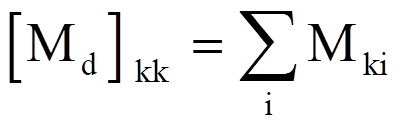 (2.6.13)
The resulted equation (2.6.13) is an explicit form and can be solved directly. It had been verified that the explicit form of the Taylor Galerkin scheme is equivalent to the Lax-wendroff finite difference scheme. The Lax-wendroff scheme is a second order time and space accuracy scheme. Also it can be written as a central difference scheme plus a second order space difference term.
2.7 Artificial viscosity
Since the explicit two-step Taylor Galerkin finite element scheme will produce an equivalent central difference scheme plus a second order difference term. Numerical analysis had proved that across the shock wave the Lax-Wendroff scheme will produce oscillate numerical results. In order to damping out the oscillation a small amount of artificial viscosity is necessary to adding into the difference equation. The artificial viscosity is added to equation (2.2.2) in the following way
 (2.7.1)
Where ART represents the artificial viscosity term bk is a gradient indicator and is defined below by equation (2.7.3). bk value can also be limited through the upper (dupr) and lower (dlow) bounded values. a is a scalar defined by the user and the value of a should be 0.0 <a<1.0.
bk = dupr, if Fk > dupr
= Fk , if dupr > Fk > dlow
= dlow, if Fk < dlow (2.7.3)
The value of Fk is calculated by the following formula :
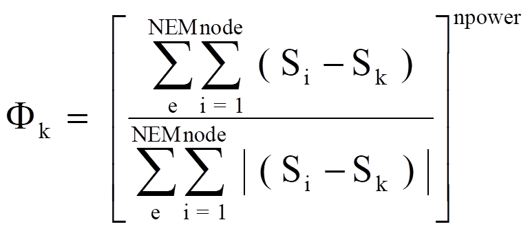 (2.7.4)
Where NEM denotes the total number of elements in the computational domain. "node" represents the total number of nodes on each element. S is a scalar variable such as pressure, density, temperature, and energy. "npower" is an integer number.
2.8 Correction of velocities on the solid surface
For inviscid flow, after the numerical calculation of equation (2.6.12) the normal velocity at the solid wall is not always zero. It can be easily seen from equation (2.6.8), that the element central velocities calculated from the first half time step do not always satisfy the normal conditions at the solid wall. It is necessary to do some numerical correction such that the normal velocity at the solid wall surface will zero. Therefore the following scheme is used to eliminate the normal velocity.

 (2.8.1)

where [U,V,W] are the corrected velocities and [U',V',W'] are the velocities calculated after the second time step.
2.9 Farfield boundary conditions
Flow variables at farfield locations can be calculated by following schemes
1. A fiction cell is created at farfield locations and flow variables at these locations are calculated as an interior point. The assigned values of flow variables at this fiction cell are based on following methods :
a. All incoming and subsonic outgoing flows: Flow variables at these fiction cell are set equal to those free stream values
c. Supersonic outflow : Flow variables at these fiction cell are set equal to those corresponding interior cell's values
2. Base on the Jameson's [1986] local one-dimensional Riemann invariant analysis
3. Same as scheme 2 but for subsonic outgoing flow, the free stream static pressure is kept as a constant.
4. Same as schemes 2 and 3 but for outgoing flow, flow variables are set equal to those corresponding interior points' values such that zero gradients will achieve at these locations.
2.10 Inviscid and Viscous Conical Flow Equations
For solving supersonic flow past a slender body problem, a space marching method can be used. The basic assumption of the space marching method is that flow properties at upstream locations will not be effected by down stream condition as long as supersonic conditions are maintained. When applying the space marching method to solve the supersonic flow problem, a starting plane solution is needed. Usually in order to obtain the starting plane solution, a conical flow assumption was made at the tip of the conical body. The conical flow assumption for inviscid flow makes use of the fact that a significant length scale is missing in the conical direction for a flow field surrounded by conical boundaries. As a result of no variation in flow properties in the radial direction, a three dimensional inviscid flow problem is reduced to a two-dimensional problem. The concept of conical flow is strictly valid only for inviscid flows. However, the viscous portions of the same flow fields have been observed in experiments to be strongly dominated by the outer inviscid conical flow. Anderson [1973] suggested that if all derivatives in the radial direction of the Navier Stokes equations are set equal to zero, then a quick estimate of the heat transfer and skin friction could be obtained. The Navier Stokes equations solved in this manner are called the conical Navier-Stokes equations. The conical Navier Stokes equations could be obtained through the transformation of the Cartesian Navier Stokes equations by letting

Then the set of partial differential equations (2.3.1) transforms to
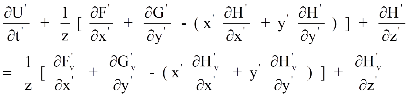 (2.10.1)
where the components of U', F', G', and H' are same as equation (2.3.1) and the viscous flux are defined by
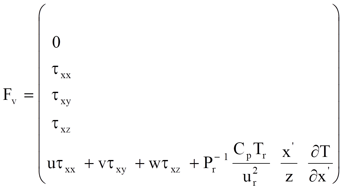
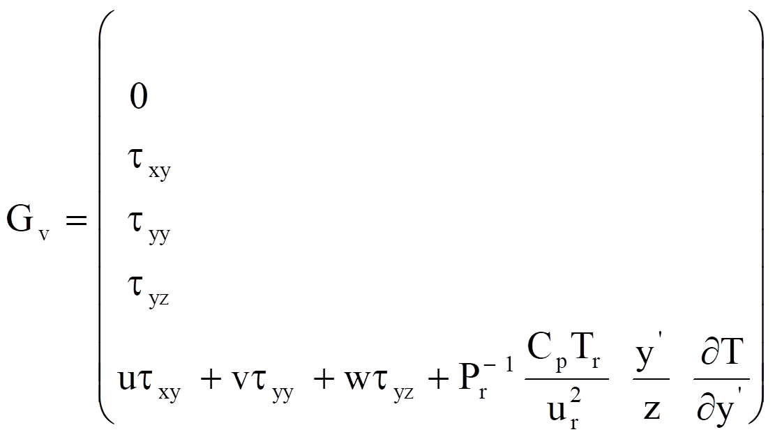
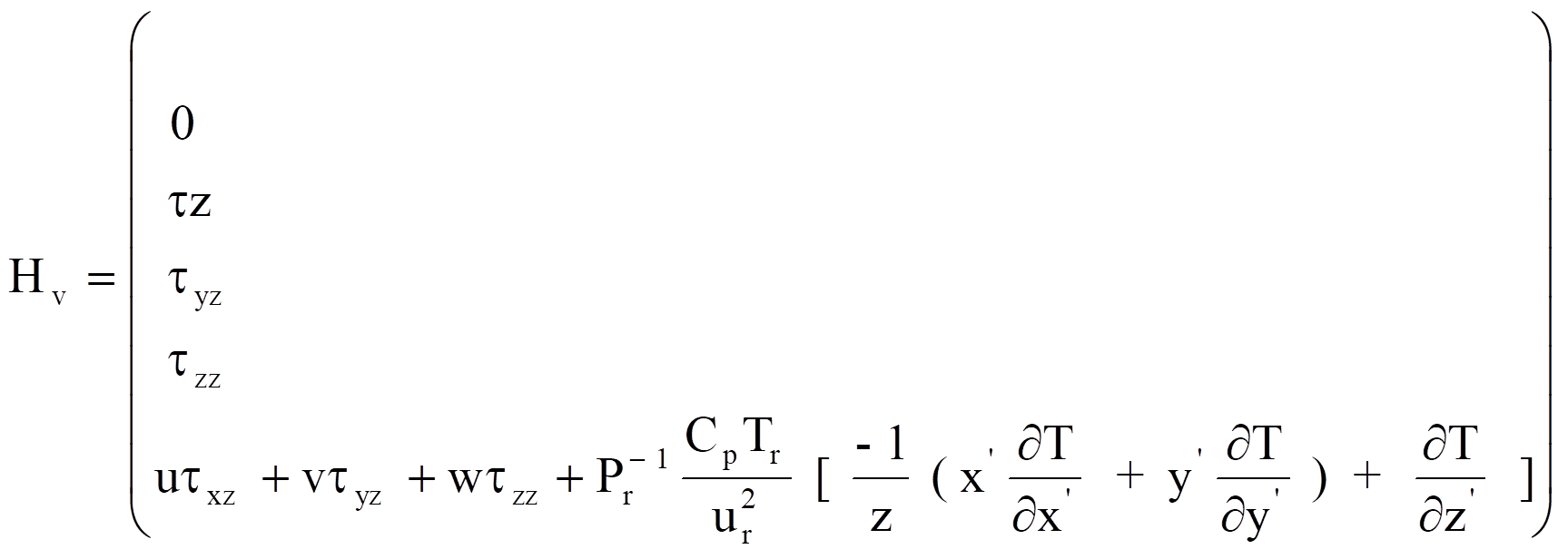
where


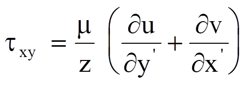


The conical flow assumption for above equation is that all derivatives in the z' direction are set equal to zero. With the conical flow assumption, the inviscid flow solutions of equation (2.10.1) are self-similar. The solution of the conical Navier Stokes equations is depend directly on the position where they computed. Currently, the FluSol program has capabilities of (1) providing the starting plane solutions for three-dimensional flow problems (2) generating a three dimensional mesh and corresponding initial and boundary conditions. When using the FluSol program to solve the three dimensional conical flow problem, user must provide a set of two dimensional meshes and the location of z coordinate and a factor value. The geometry coordinates in the FluSol program for conical flow problems are defined as

Where factor is a scale factor provided by the user. Also if more than two sets of (z , factor) are provided, the FluSol program will perform the space marching procedure. In other words, to solve a true three dimensional problem users must provide all z coordinates and factor values. FluSol program will solve the first set of (z,factor) problem by using the conical flow assumption. Then FluSol will generate a three dimensional mesh, based on the rest set of (z,factor), and corresponding initial and boundary conditions.
2.11 Governing Equations for Two Dimensional Axisymmetrical Flow
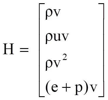
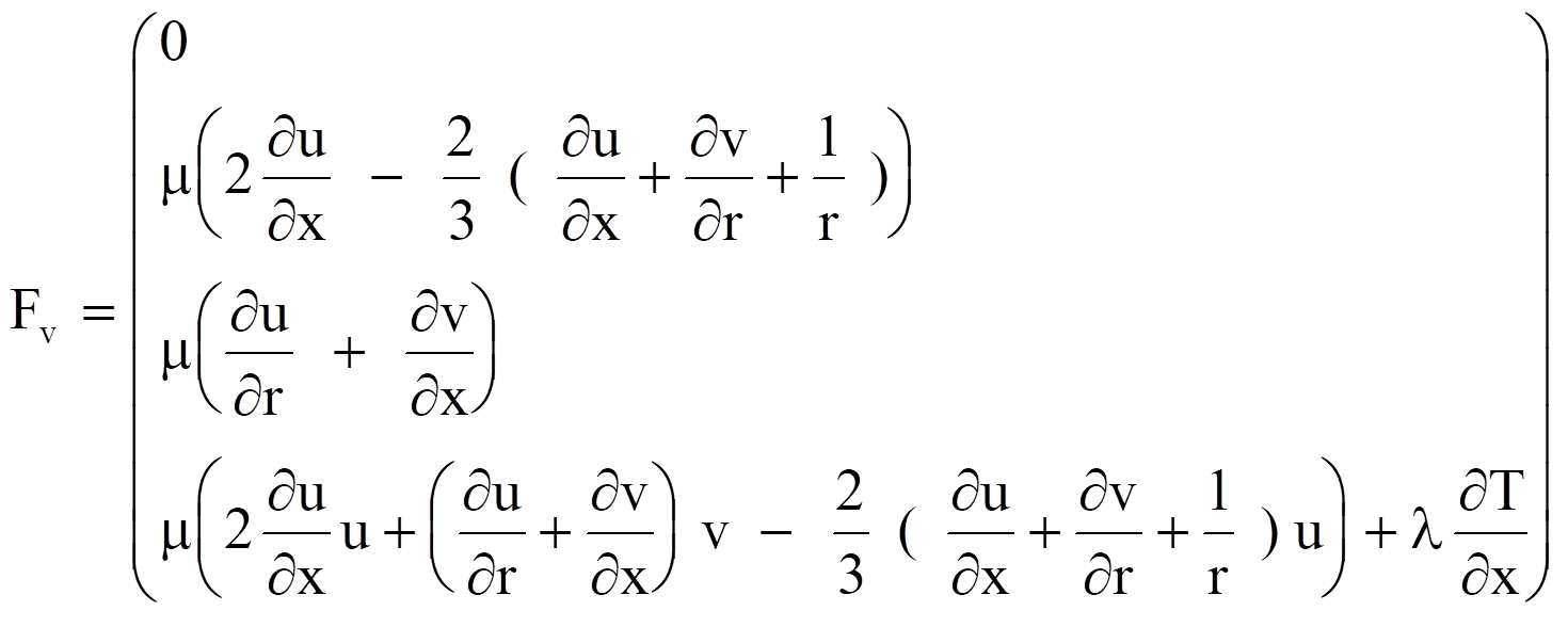
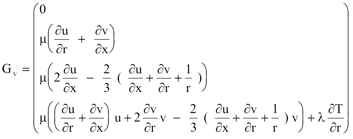
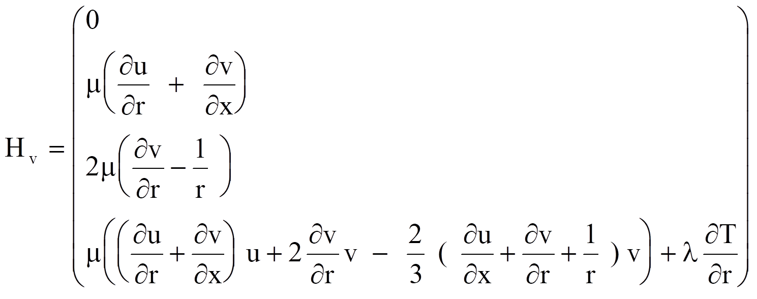
For axisymmetrical flow problems, the governing equations (2.3.1) can be rewritten in the following cylindrical coordinate form
 (2.11.1)
where
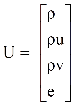
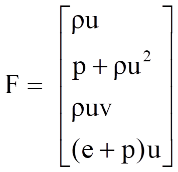
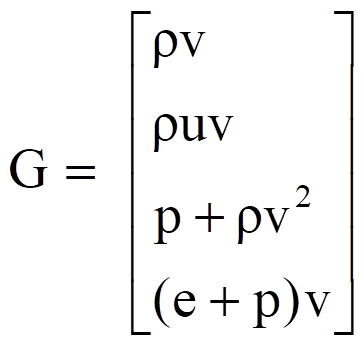
Also equation (2.11.1) can be further simplified into the following general form of equation for one dimensional flow problems.
 (2.11.2)
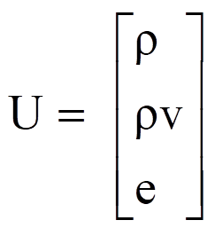
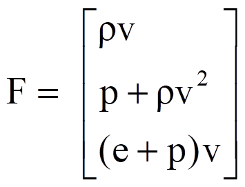
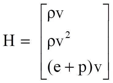
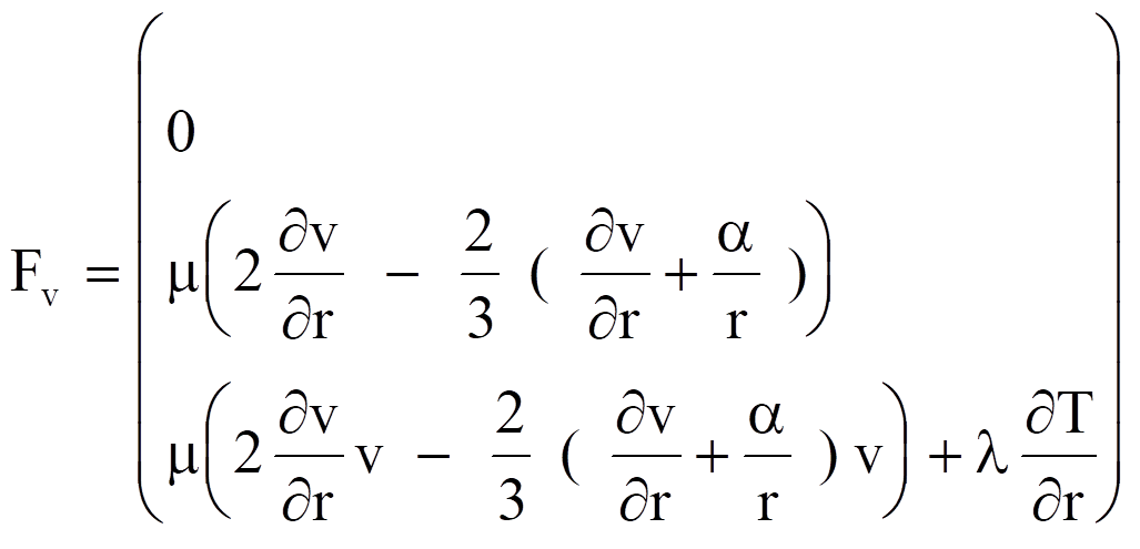
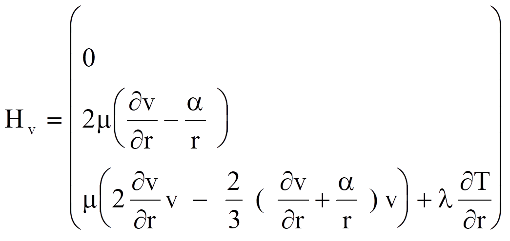
where a = 0, 1, 2 represents the Plannar, cylindrical, and spherical coordinates.
2.12 The B.V.L.R. Method
The B.V.L.R. method is a short description of the numerical method developed by Babenko, Voskresenskii, Lyubimov and Rusanov et al 1961, 1963, 1967. This method was first developed for pure supersonic flows but was later modified by Rusanov 1968 and Lyubimov and Rusanov 1970 to solve mixed subsonic-supersonic flow problems. A full description of the B.V.L.R. method can be found in the book "Numerical Methods in Fluid Dynamics" edited by Maurice Holt. Currently, the FluSol program can only solve 2D and axisymmetric supersonic flow problems.
2.13 Governing equations for the mixture flow of gas and solid particles
FluSul can solve the solid particle and the gas mixture flow problems. There are two kinds of approach to solve the particle and the gas mixture flow problems. The first is the Eulerian approach and the second is the Lagrangian approach. In the Eulerian approach both the particle and the gas phases are treated as continuum medium. In the Lagrangian approach, the particles are divided into many groups. Each group contains many particles of the same flow properties. Then the trajectory of each group of particles is traced. The temperature, velocities and locations of each group are recorded for calculating drag force and heat transfer between the particles and the gas.
To formulate the governing equations for the particle and the gas mixture flow, it has been assumed that :
1. The particles are assumed to be spheres.
2. For the Eulerian approach the number density of the particle is assumed to be large, so that the particle flow can be treated as a continuum.
3. The volume occupied by the particles is neglected and the particles do not contributed to the pressure.
4. There is no interaction between particles.
5. The temperature is uniform within each particle.
2.13.1 Eulerian Approach For Both Particle And Gas Flow
With the above assumptions, the conservation equations for the particle and the gas mixture flow with chemical reaction can be written as follows, Chang and Sichel :
 (2.13.1)
Where U, F, G, Fv, Gv, Hv are the gas conservative flow variables, inviscid flux and viscous flux terms and are defined in section 2.1. The source term Sg due to the presence of the particles is written as follow :
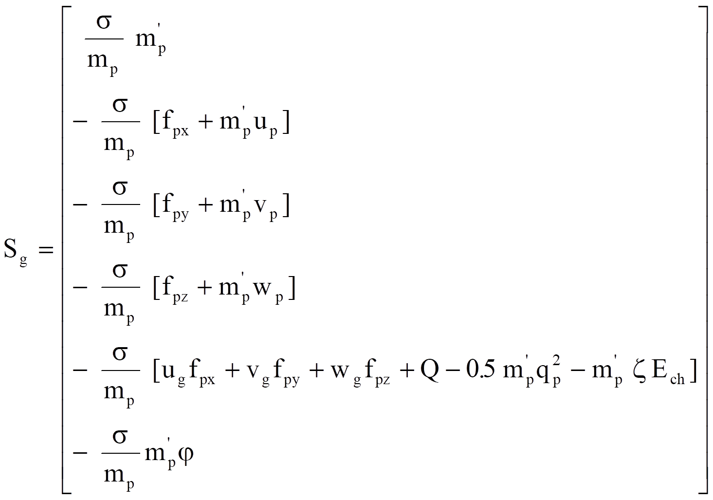 (2.13.2)
Where s and
mp are the particle concentration and the mass of single of
particle.  is the ratio of oxygen
being consumed per unit mass of particle. x
is the fraction of chemical energy Ech
released by the burning of solid particle used to heat up the gas flow. fpx, fpy , fpz and Q are the
drag force and the rate of heat transfer from the gas to an individual
particle. fpx,
fpy , fpz and Q are given by :
fpx = 0.125 pd2 r(ug-up)Dq Cd
fpy = 0.125 pd2 r(vg-vp)Dq Cd (2.13.3)
fpz = 0.125 pd2 r(wg-wp)Dq Cd
Q = dmCp (Tg-Tp)( Nu/ Pr)
Where C p and N u are the drag force coefficient and the Nusset number. The empirical relations of Henderson were used for the drag force coefficient and the Nusset number is taken from Knudsen and Katz by :
Nu = 2.0+0.6Re1/2 Pr1/3 (2.13.4)
Dq is the velocity difference between the gas and the particle and is defined by :
Dq = [ (ug - up) 2+(vg - vp) 2+(wg - wp) 2 ]1/2 (2.13.5)
mp is the mass of a single particle mp = 1/6 rp pd 3 . mp’ is the rate of change of mass for a single particle due to the chemical reaction of solid surface. The particle phase equations can be written as follow :
 (2.13.6)
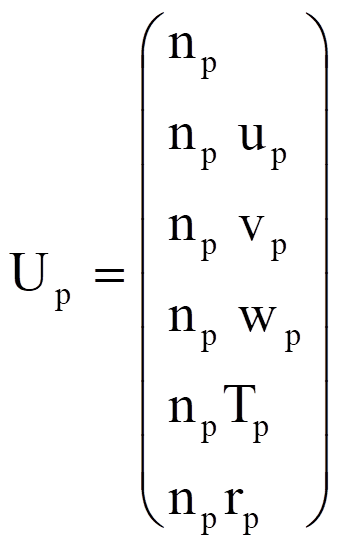
Where Up is the particle flow variable. Fp, Gp and Hp are the flux terms and Sp is the source term. Up, Fp, Gp, Hp and Sp are defined as follows :
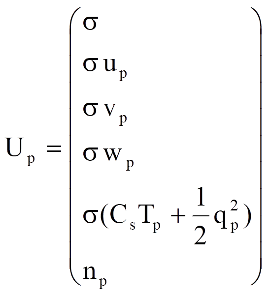
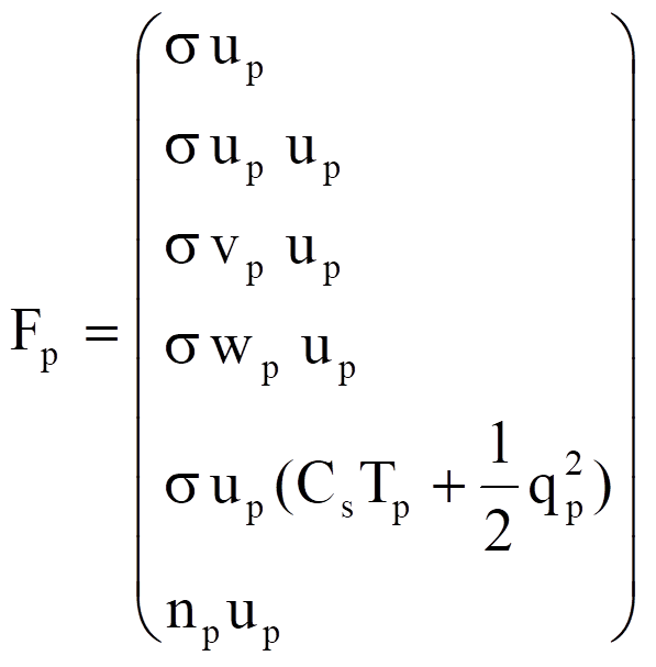
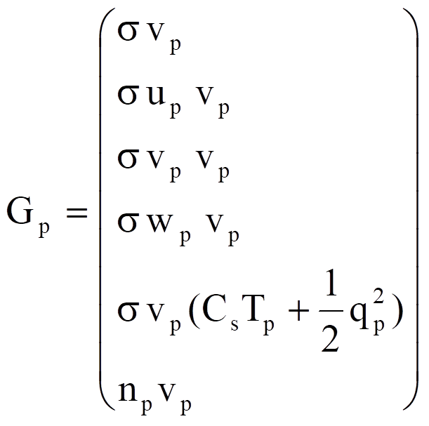
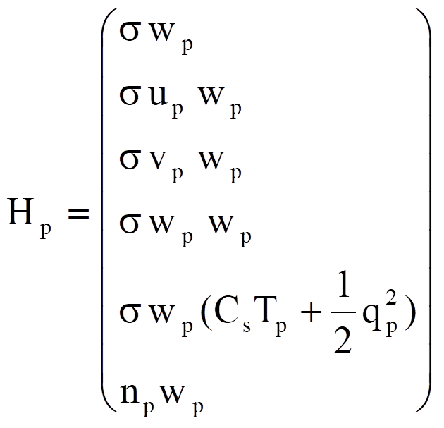 (2.13.6)
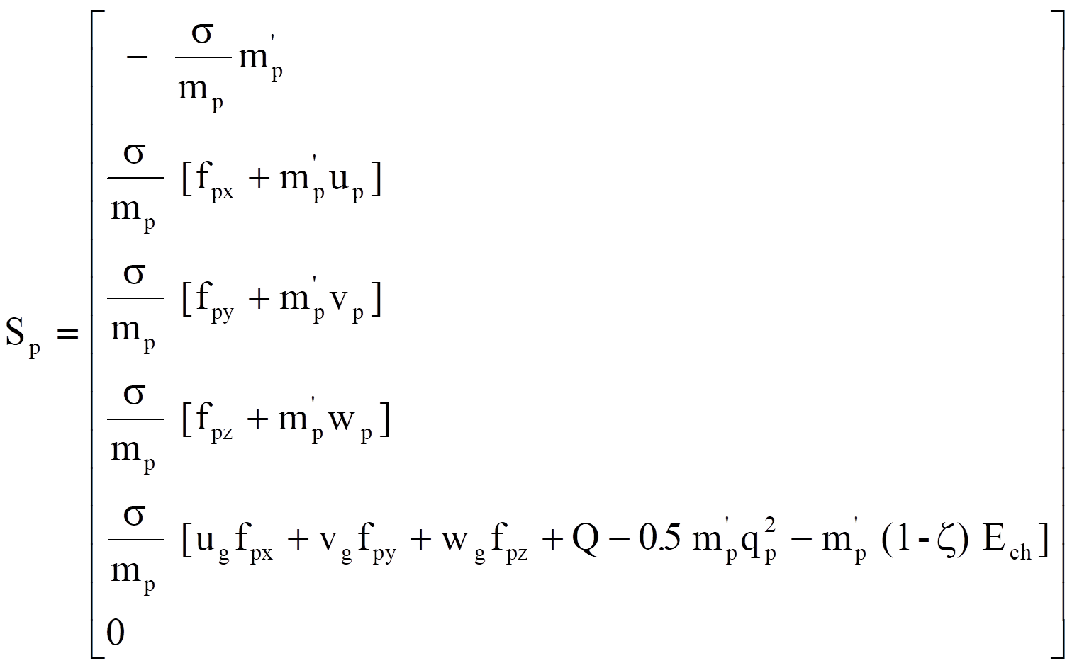
np is the number density of the particle flow. If there is no chemical reaction between the gas and the particles then the number density equation is equivalent to the particle concentration equation
If the solid particles are not inert and chemical reaction may occur due to the high temperature spot in the flow field, then the radius of the particle will be changed. It is necessary to re-write the above equations in terms of the particle radius such that the change of particle radius can be solved directly. Therefore, the equation (2.13.6) will be written as follows:
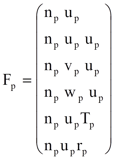
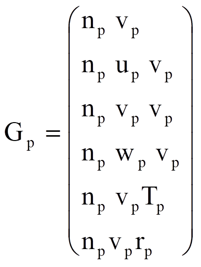
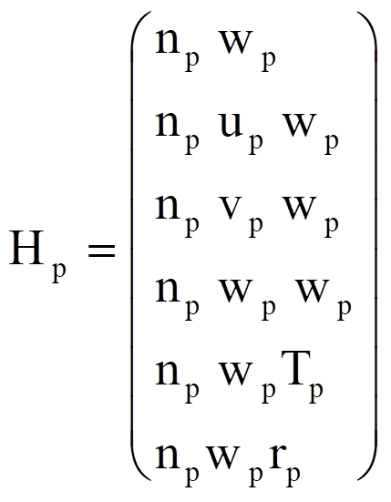
 (2.13.7)
If there is not chemical reaction between the particles and the gases, then the particle number density equation will be equivalent to the particle radius equation.
2.13.2 The Lagrangian Approach For Particle Flow
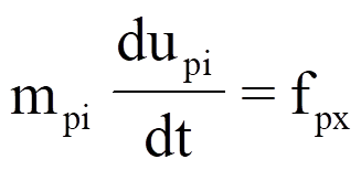
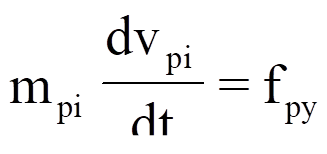
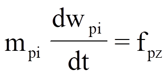
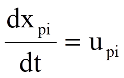
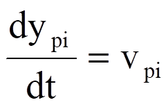
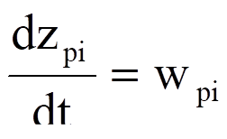
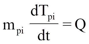
In the Lagrangian approach, each individual particle represents a group or fixed number of particles and its location is traced during each calculation. The temperature, velocities and material properties of each group of particle is recorded for calculating the drag force and heat transfer between the particle and the gas. The trajectory, the equation of motion, and the energy equation for i-th group of particles can be written as follows :
 + mpi
g lx (2.13.8)
 + mpi
g ly (2.13.9)
 + mpi
g lz (2.13.10)
 (2.13.11)
 (2.13.12)
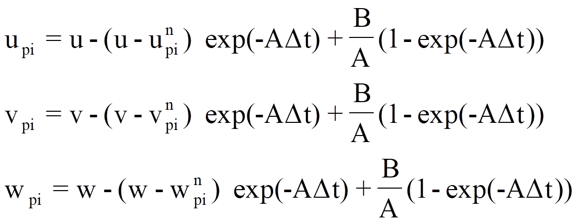
Where fpx, fpy, fpz, and Q are defined by equation (2.13.3). g is the gravity constant and lx, ly, and lz are the directional cosine of the gravity vector. The numerical method used to solve the above particle equation is taken from Sharam. Sharma assumed that the Reynolds number and the drag coefficient are constant during a small time step Dt. Under these assumptions, the particle equations can be integrated analytically as following :
 (2.13.13)
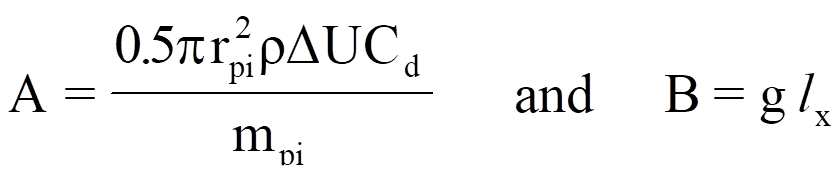 , g ly, or
g lz
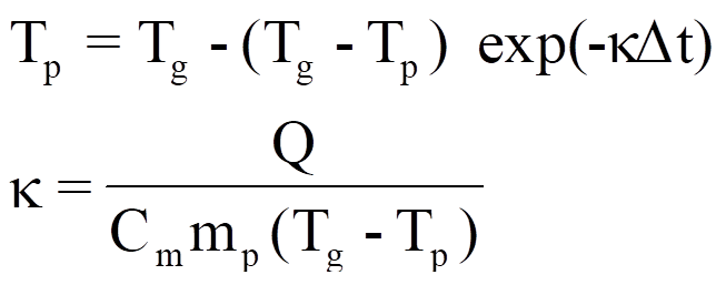 (2.13.14)
The trajectory of i-th group of particles can be calculated from :
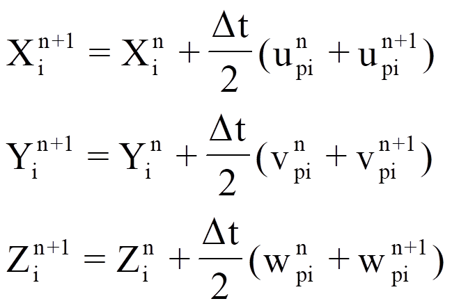 (2.13.15)
References
Bird, R.B., Stewart, W.E. and Lightfrot, E.N., Transport Phenomena, John Wiley & Sons, New York, 1960.
Jameson, A., Schmidt, W. and Turkel, E., "Numerical Solution of the Euler Equations by Finite Volume Method Using Rung-Kutta Time Stepping Schemes", AIAA Paper 81-1259, 1981.
Jameson, A. and Yoon, S., "Multigrid Solution of the Euler Equations Using Implicit Schemes," AIAA Journal, vol.24, no.11, Nov. 1986, pp.1737-1743.
Kee, R.J., Dixon-Lewis, G., Warnatz, J., Coltrin, M. E. and Miller, J.A., "A Fortran Computer Code Package for the Evaluation of Gas-phase Multicomponent Transport Properties," Sandia national Laboratories report, SAND 86-8246, 1986.
Kee, R.J., Rupley, F.M. and Miller, J.A., "Chemkin-II: A Fortran Chemical Kinetics Package for the Analysis of Gas Phase Chemical Kinetics," Sandia national Laboratories Report, SAND89-8009B, 1991.
Marcum, D.L. and Hoffman, J.D., "Numerical Boundary Condition Procedure for Euler Solvers," AIAA Journal vol.25, No.8, pp.1064-1072, Aug.1987.
Warnatz, J., "Influence of Transport Models and Boundary Conditions on Flame structure," Numerical Methods in Flame propagation, Eds. N. Peters and J. Warnatz, Friedr. Vieweg and Sohn, Wiesbaden, 1982.
Wilke, C.R., "A Viscosity Equation for Gas Mixtures," J. Chem. Phys., 18, pp.517, 1950.
Holt, M., Numerical Methods in Fluid Dynamics, Spring-Verlag 1984.
Babenko, K.I., Voskresenskii, G.P. ; USSR Comp. Math. Math. Phys. 1 (1961).
Babenko, K.I., Voskresenskii, G.P., Lyubimov, A.N., Rusanov, V.V.: Three Dimensional Flow of Ideal Gases around Smooth Bodies. NASA TT F-380, 1968.
Lyubimov, A.N., Rusanov, V.V.: Gas Flows Past Blunt Bodies, Part.1. NASA TT F-714, 1973.
Hirschfelder, J.O., Curtiss, C.F. and Bird, R.B., Molecular Theory of Gases and Liquids, John Wiley & Son, New York, 1954.
Chang, F.L. and Sichel, M.,”Analytical and Numerical Study of Shock Wave Propagation in a Non-Uniform Dusty-Gas Mixture Layer”,Fall technical Meeting, Eastern Section of Combustion Institute, San Juan, Puerto Rico, December, 1986.
Chang, F.L. and Sichel, M.,”Numerical Simulation of Normal Shock Wave Reflection in the Dusty-Gas Mixtures”, technical Meeting on the Central Section of the Combustion Institute, May 5-6, 1986, Cleveland, OH.
Crowe, C.T., Sharma, M.P. and Stock, D.E.,”The Particle-Source-In-Cell (PSI-CELL) Model for Gas-Droplet Flows”, J. Fluids Eng., June, 1977, pp.325.